Using SamplePipeline
A sample-level (patient-level) visualization of the gene and cell-type of interest.
First, the data and package are loaded. This may take a minute. Set your gene of interest (GOI) here!
[77]:
%%time
import sys, os
sys.path.append(os.path.dirname(sys.path[0]))
from importlib import reload
import genereporter.sample_pipeline as spModule
reload(spModule)

sp = spModule.SamplePipeline(
    wdir=os.path.dirname(sys.path[0]), adata="data/output/adata.h5ad", anonymous = True)

sp.adata
CPU times: user 62.7 ms, sys: 256 ms, total: 319 ms
Wall time: 547 ms
[77]:
AnnData object with n_obs × n_vars = 5397 × 16719
    obs: 'sampleID', 'barcode', 'n_genes_by_counts', 'log1p_n_genes_by_counts', 'total_counts', 'log1p_total_counts', 'pct_counts_in_top_20_genes', 'total_counts_mt', 'log1p_total_counts_mt', 'pct_counts_mt', 'total_counts_ribo', 'log1p_total_counts_ribo', 'pct_counts_ribo', 'total_counts_hb', 'log1p_total_counts_hb', 'pct_counts_hb', 'outlier', 'mt_outlier', '_scvi_batch', '_scvi_labels', 'leiden_res0_6', 'manual_celltype_annotation', 'celltypist_cell_label', 'celltypist_conf_score', 'celltypist_cell_label_coarse'
    var: 'n_cells', 'highly_variable', 'means', 'dispersions', 'dispersions_norm'
    uns: '_scvi_manager_uuid', '_scvi_uuid', 'celltypist_cell_label_coarse_colors', 'celltypist_cell_label_colors', 'hvg', 'leiden', 'leiden_res0_6_colors', 'neighbors', 'pca', 'sampleID_colors', 'umap'
    obsm: 'X_pca', 'X_scVI', 'X_umap'
    varm: 'PCs'
    layers: 'int_norm', 'log_int_norm', 'log_norm', 'norm', 'raw'
    obsp: 'connectivities', 'distances'
[74]:
GOI = 'ACTG2' # set the GOI!!!

CELL_TYPE_COL = 'manual_celltype_annotation'

SAMPLE_COL = 'sampleID'
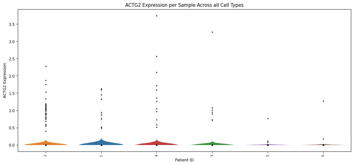
Violin plot for each sample’s expression distribution, across all cell types for the gene of interest. A scatterplot of each sample is overlayed to show the individual cells. This is particularly useful to quickly identify samples that perhaps have a very low number of cells.
[75]:
sp.pl_violin(GOI, cell_type_col = CELL_TYPE_COL, sample_col = SAMPLE_COL)
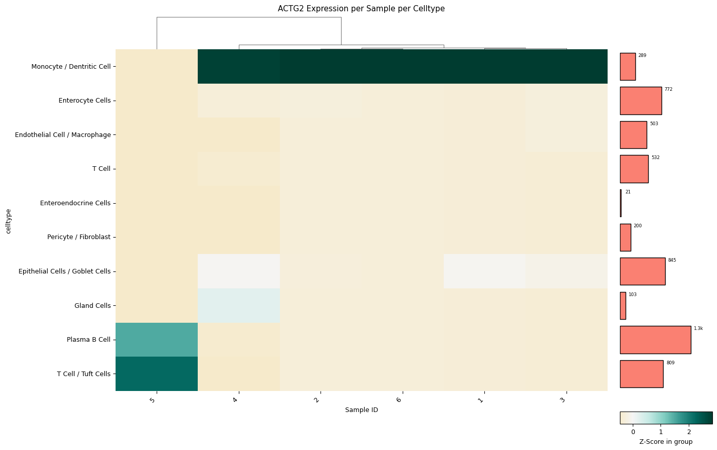
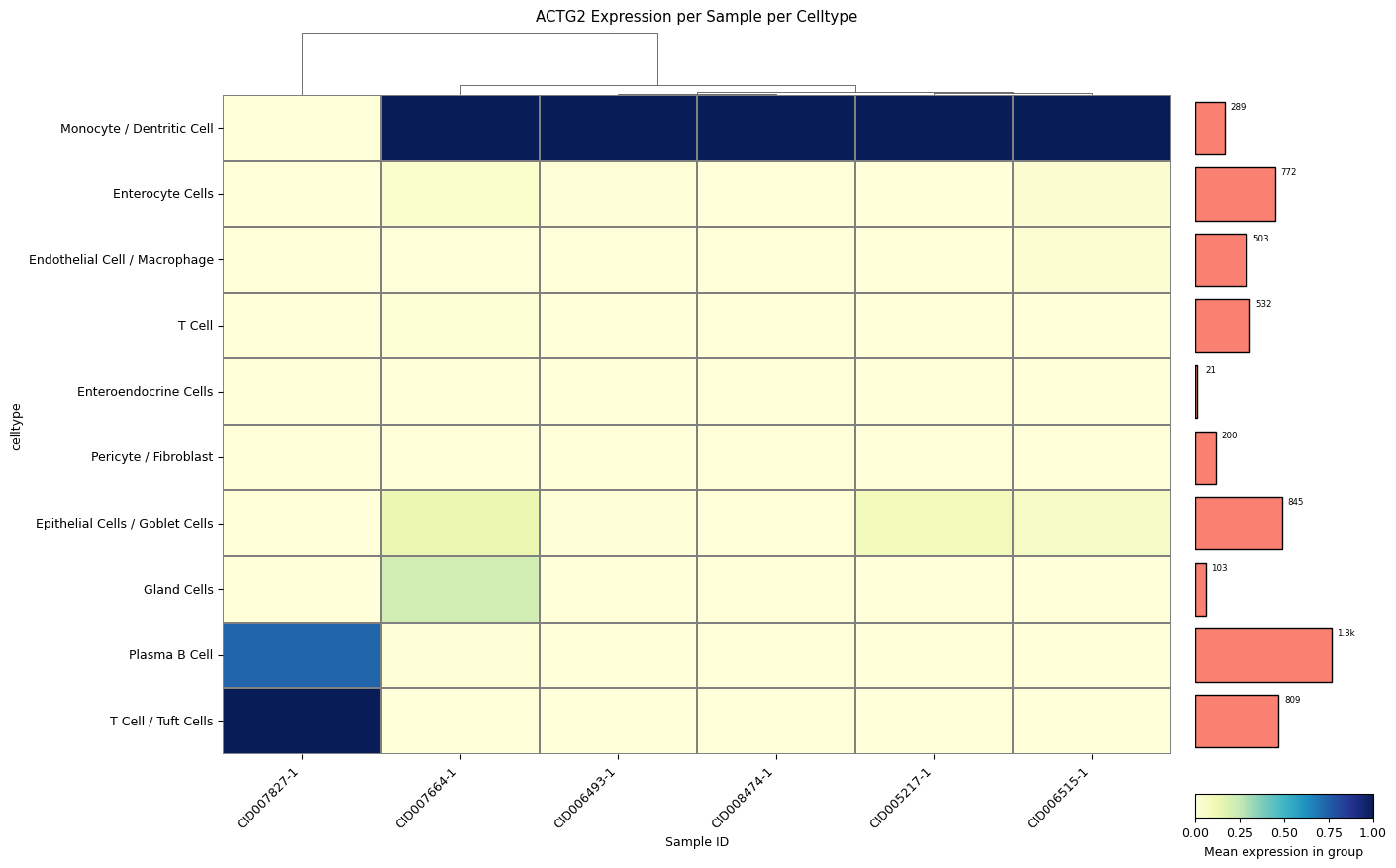
A clustermap (hierarchically clustered heatmap) across all samples for all cell types. The mean expression values are either standardized between 0 and 1 for each patient or z-score normalized. The choice between standard scaling and z-score normalization depends on the specific analysis objectives and the presence of outliers within the data. Standard scaling provides a straightforward representation of mean expression values, while z-score normalization offers robustness against outliers, albeit at the expense of directly showing mean expression values. The user can quickly change which version is created with a single method parameter: z_score=0 for z-score normalization by each row (cell type), z_score=1 for z-score normalization by each column (patient), or z_score=False for standard scaling by each column (patient).
[76]:
sp.pl_sample_celltype(GOI='ACTG2', z_score=1, cell_type_col = CELL_TYPE_COL, sample_col = SAMPLE_COL)
[67]:
sp.pl_sample_celltype(GOI='ACTG2', z_score=0, cell_type_col = CELL_TYPE_COL, sample_col = SAMPLE_COL)
Clustering failed: The condensed distance matrix must contain only finite values.
Falling back to no clustering
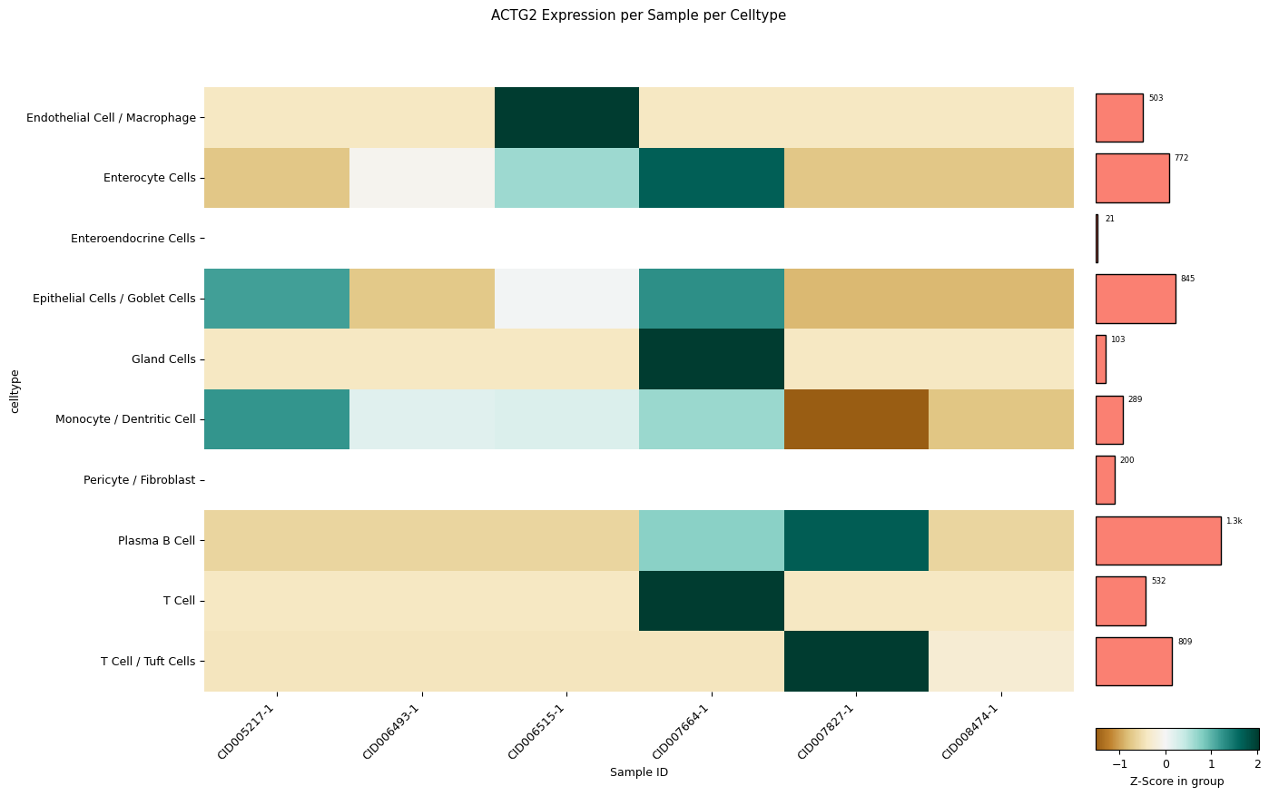
[68]:
sp.pl_sample_celltype("ACTG2", z_score=None, cell_type_col = CELL_TYPE_COL, sample_col = SAMPLE_COL) # balanced data set
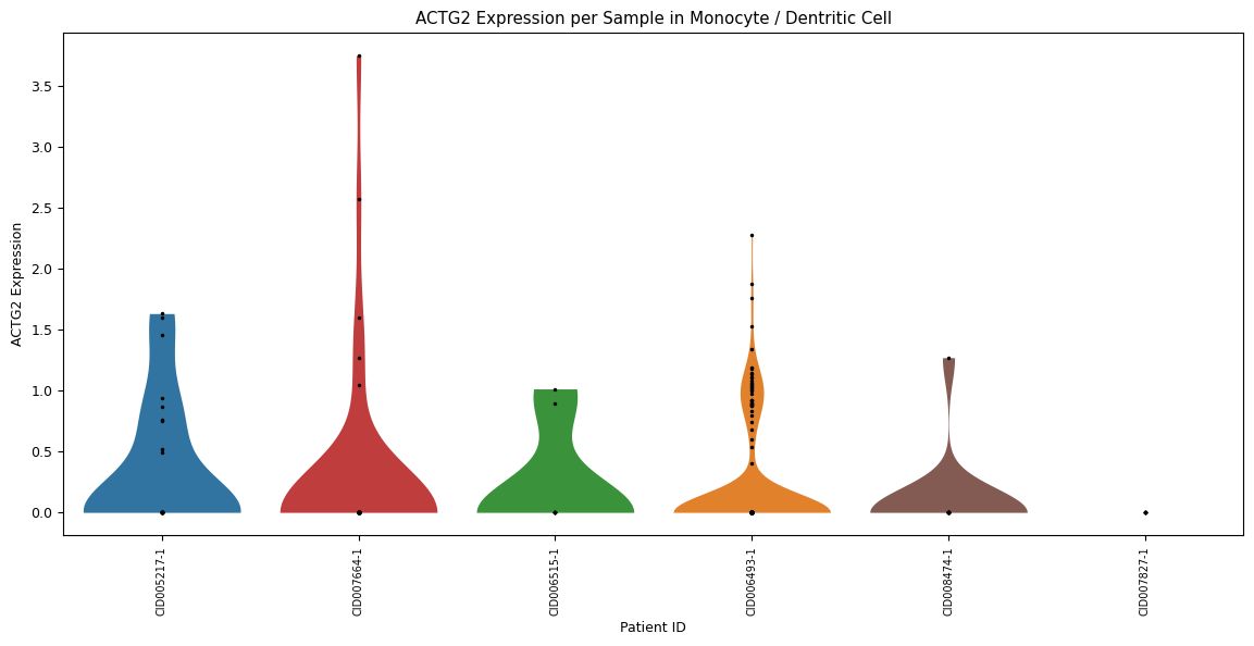
Zooming further in, a violin plot across all samples in one specific cell type (instead of over all cell types). Set this cell type using the parameter
celltype=’[your celltype here]’
[69]:
sp.pl_violin(GOI, celltype='Monocyte / Dentritic Cell', cell_type_col = CELL_TYPE_COL, sample_col = SAMPLE_COL)